Lab 01 – Reproducible research with R Markdown and GitHub

This week’s lab provides you with a general introduction to the tools and platforms we use during the semester, which are R, RStudio Server, and GitHub. R is the name of the programming language itself and RStudio Server is a convenient interface that you access using a web browser at https://rstudio.cos.gmu.edu.

Obtaining your starter code

Since this is the first time that you will obtain starter code for a lab, we will take the time to go through the procedure step-by-step. Carefully follow the instructions provided below and do your best to understand why you’re performing each step, as you will follow a similar series of steps every time you are assigned a new lab report!

Login to RStudio Server

Navigate to the class installation of RStudio Server using this link https://rstudio.cos.gmu.edu and login using your username and password. After logging in, you will be presented with an interface that looks something like this,

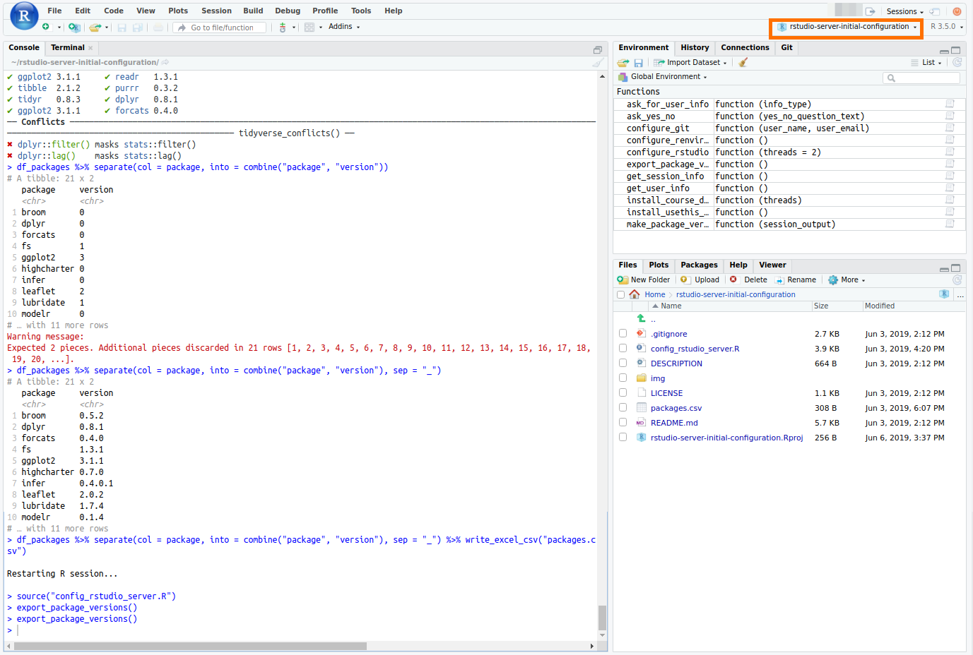
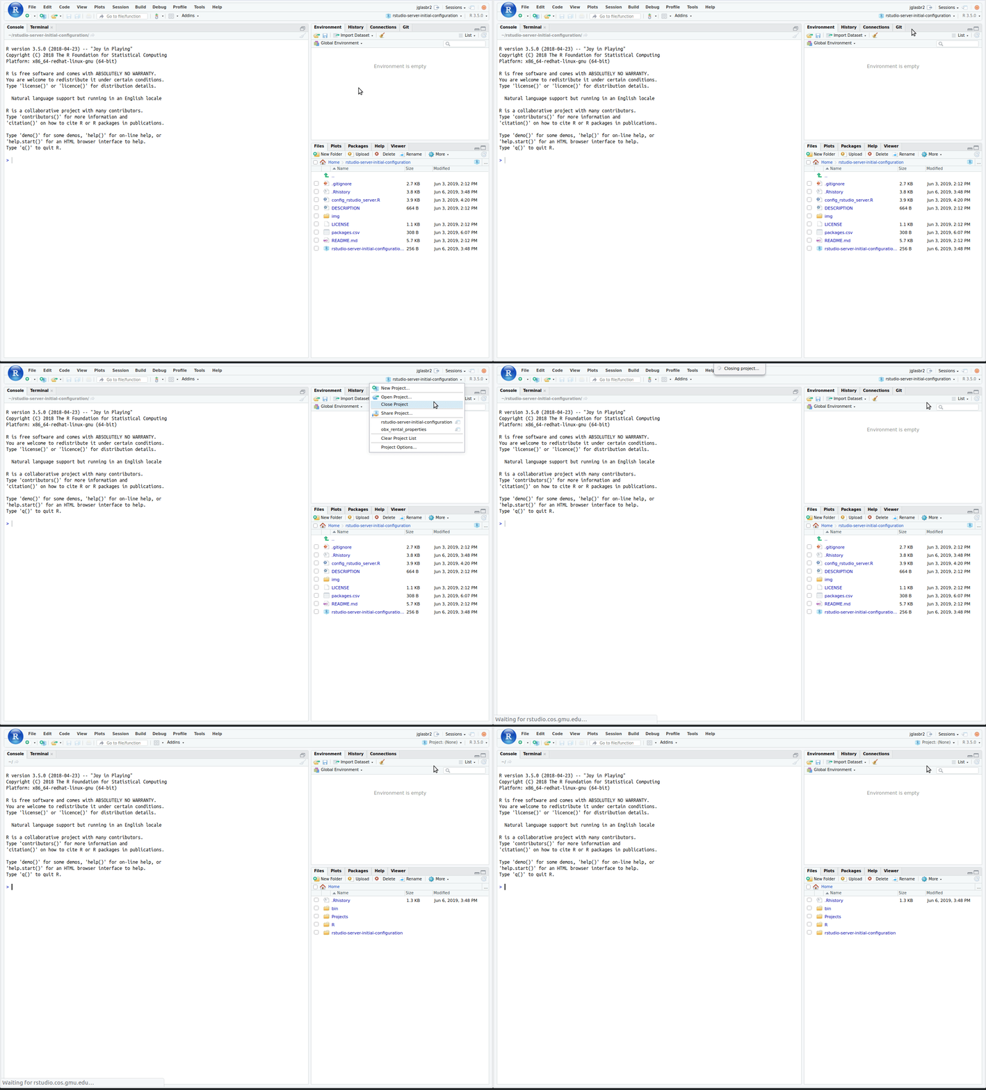
If, as shown in the above image, you see the phrase rstudio-server-initial-configuration in the region surrounded by the orange rectangle, then that means you still have the initial configuration workspace activated. To close it, click rstudio-server-initial-configuration and then click Close Project,

Accept GitHub Classroom assignment

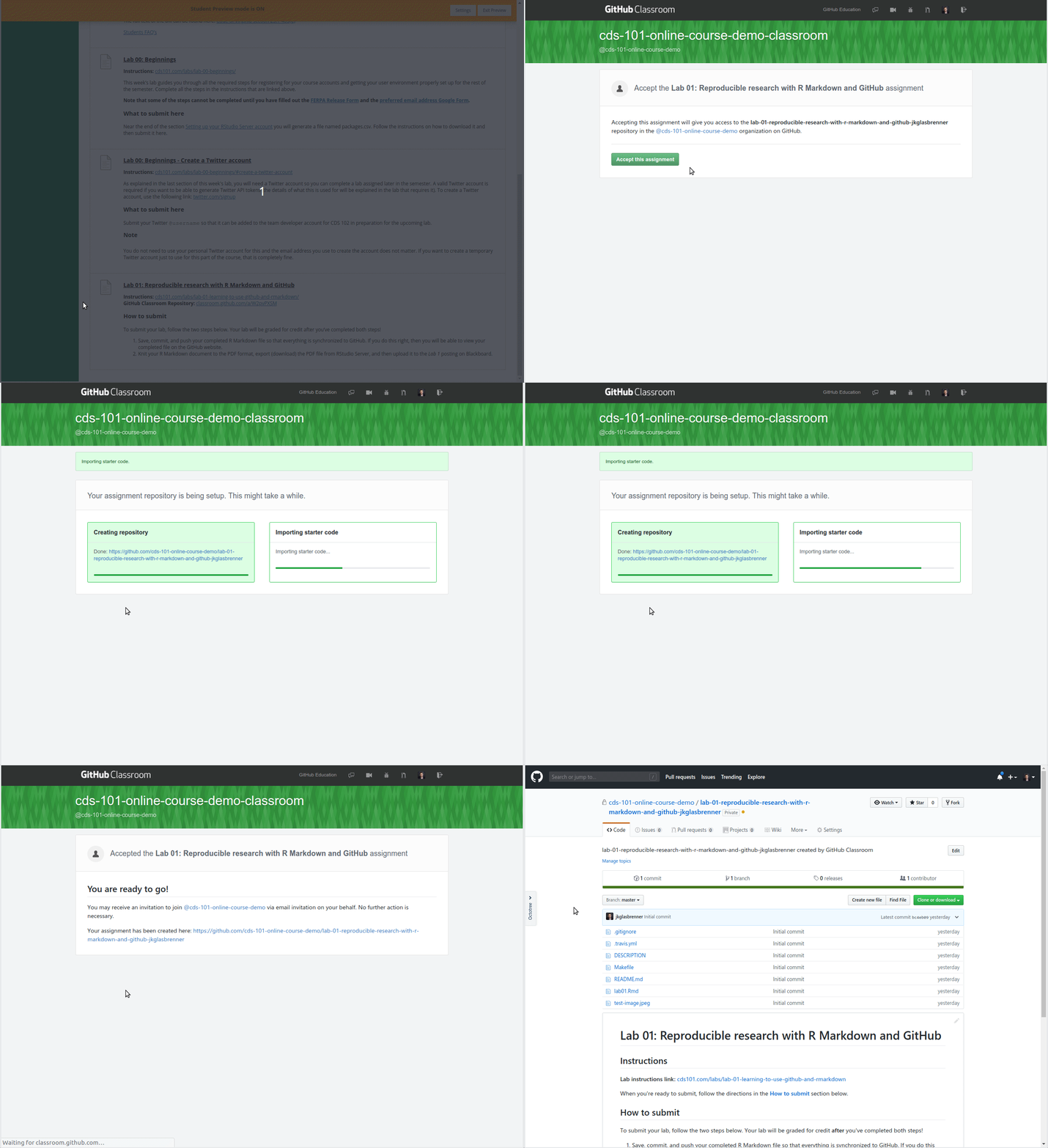
Each time you are assigned a lab to complete for the course you will need to get a copy of the starter code on GitHub. Copies are distributed using GitHub Classroom. As a student, all you need to do to grab your personal copy is click a link and then click a button to “accept” the assignment.

To accept the starter code for Lab 01, open a new tab in your web browser and go to the Blackboard page for CDS 102. Click the Labs link on the left sidebar, locate the Lab 01 assignment, and click the GitHub Classroom link posted there. After following the link, if you are presented with a list of names, find yours and click it. Afterwards, click accept and wait for the copying process to finish. Once copying is complete, click the final link provided to you to view your starter code.

See the animation below for an example of what this process looks like start to finish,

Clone repository to RStudio Server

The starter code that you are looking at is stored in what’s called a repository. GitHub describes a repository as follows,

A repository is the most basic element of GitHub. They’re easiest to imagine as a project’s folder. A repository contains all of the project files (including documentation), and stores each file’s revision history. Repositories can have multiple collaborators and can be either public or private.

— GitHub Glossary

Looking at the repository page is a good way to check what files are visible to course instructor and, for any group-based assignments, your teammates.

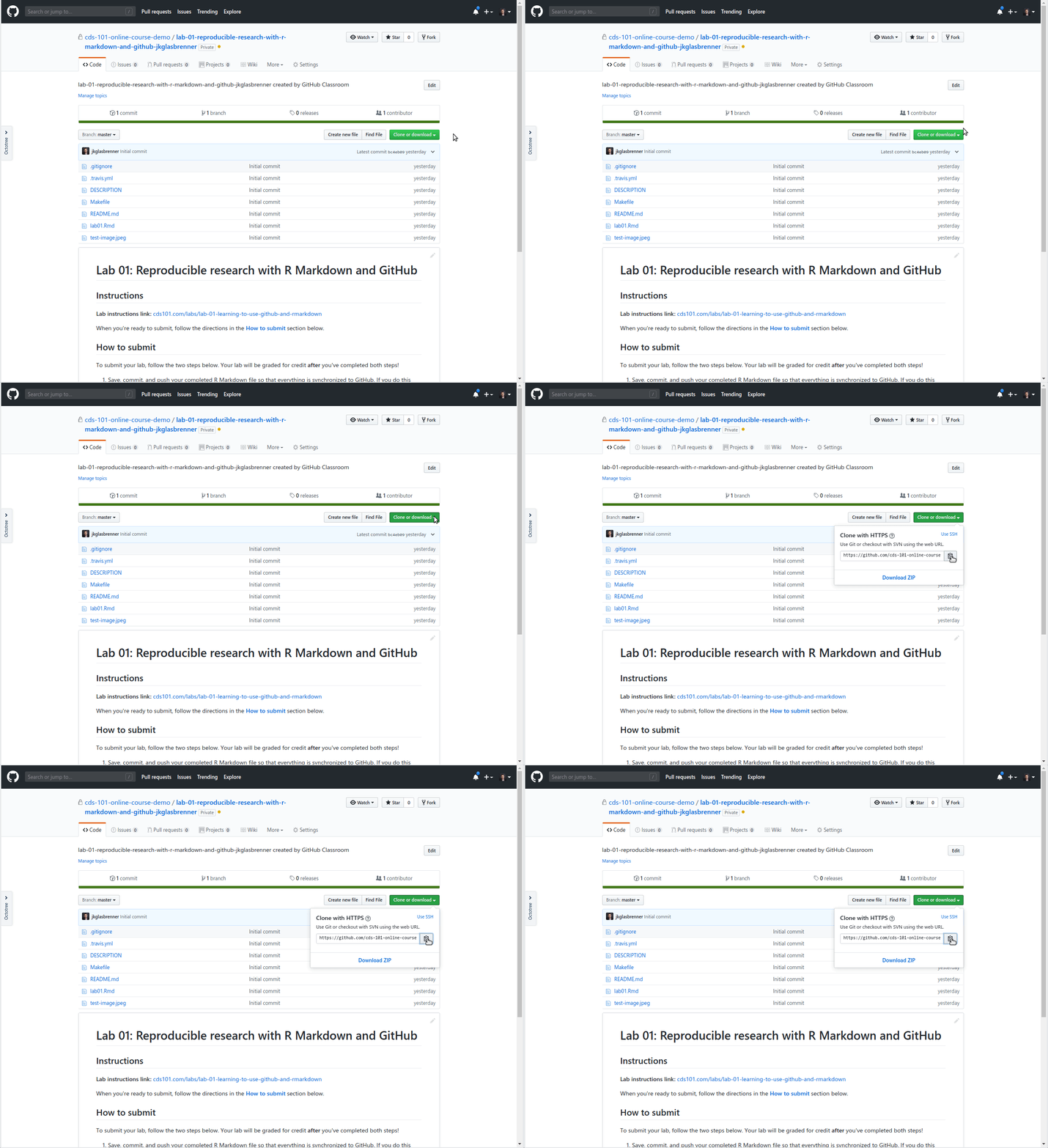
To use this starter code to complete your lab, we need a way to copy it into your RStudio Server account. The process of making an exact copy of the repository is called cloning. To clone your starter code to RStudio Server, we first click the green Clone or download button. Verify that the pop-up says Clone with HTTPS. If it does not, fix this by clicking on the blue “use HTTPS” button on the top right of the pop-up box. Finally, click the clipboard icon on the right of the pop-up to copy the link so that you can paste it elsewhere.

See the animation below for an example of what this process looks like start to finish,

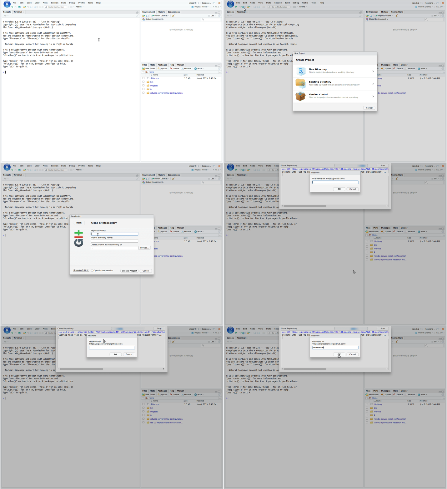
We’re almost done! The final steps you need to complete are similar to what you had to do in Lab 00. Go back to your RStudio Server tab in your web browser and look for an icon with a blue cube and plus sign near the top left of the interface. This is the New Project icon. Click the icon, then Version Control, then Git, paste the link you copied into the Repository URL box, and finally click Create Project. You will be asked to enter your GitHub username and password. If you enter the information correctly, RStudio Server will connect to GitHub and clone the repository directly into your account, and the screen will refresh.

See the animation below for an example of what this process looks like start to finish,

Quick tour of the RStudio Server interface

Now that you have your starter files cloned to your RStudio Server account, let’s get better acquainted with RStudio Server’s interface. Let’s start by opening up the file you’ll be using to complete your lab report. Look at the list of files in the lower-right panel and click the file named lab01.Rmd. Your interface should now look something like this,

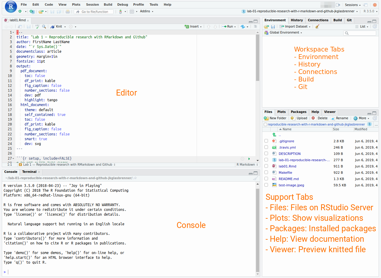
The above image labels the four default panels for RStudio Server, which are,

• Editor panel (upper-left): This is the panel where you’ll do most of your work. It is similar to plain text editors like Notepad or TextEdit that you may have installed on your personal computer or laptop. This is the place where you will complete exercises and write R code.

• Console panel (lower-left): This is the panel where you can enter different R commands. The > symbol is called the prompt, which is really just a request for an R command. When you want to test an R command but not necessarily save it to a file, this is the place to do it.

• Workspace Tabs panel (upper-right): This is the panel that provides you with information about your current workspace. The most important tabs for you to know are the Environment tab, which tells you the variables and commands you’ve defined so far, the History tab, which provides a command history, and the Git tab, which provides you with information about changes you make to your GitHub repository.

• Support Tabs panel (lower-right): This is the panel that provides you with ways to manage your files, preview images and documents, and get help.

How to switch between labs

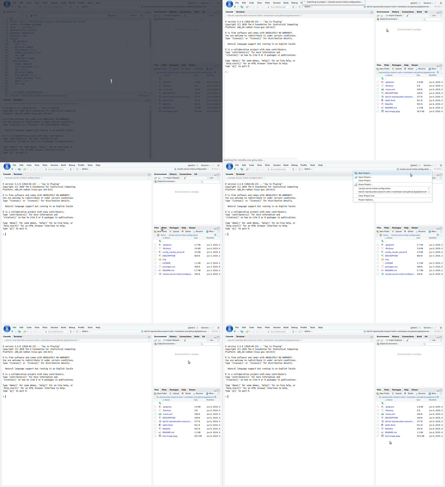
As far as RStudio Server is concerned, each lab that you work on is a separate project and is stored within its own folder. This might be different from how you like to organize files on your own computer. The advantage to this folder-based method is that files related to a specific assignment are grouped together. At the same time, browsing between many folders can become a hassle. To help with this, RStudio provides a quick way to switch between projects. To switch to a different project, click the active project name in the upper-right corner of the interface to open up a menu. Under the Share Project option is a list of the most recent projects you’ve activated. Select the project you want to work on and wait for the refresh to complete. The files listed in the lower-right panel should have changed to match the project you just activated.

The animation below demonstrates how to switch back and forth between two different projects.

Getting familiar with R Markdown

Now that you’ve obtained your starter code from GitHub and opened it in RStudio Server, we can start learning about the R Markdown format. Let’s start by taking a moment to watch the following video that summarizes what R Markdown is all about,

As you can see, the combination of R Markdown and RStudio Server allows us to combine text processing with the ability to execute code written in R. However, unlike software like Microsoft Word, there aren’t any formatting buttons for doing things like creating bold or italicized text. So how can you format your text? R Markdown does this using symbols that stand for different types of text markups. For example, typing **bold text** in a R Markdown file signals you want the words “bold text” to be bolded. Paragraphs are separated by a blank line, for example:

This is the end of the first paragraph.

This starts the next paragraph.
However, putting a line right below it will not start a new paragraph.

Let’s practice by typing in some examples!

1. Fill in your name at the top of the lab01.Rmd file if you haven’t already. Then, below ## Exercise 1, write

   ## Exercise 1
   
   This is Exercise 1.

   Save your document by clicking the save icon. Next, click the far-right side of the “knit” icon just above the editing window. In the drop-down menu that appears, choose knit to PDF. If you are asked to install updates, click Yes.

   

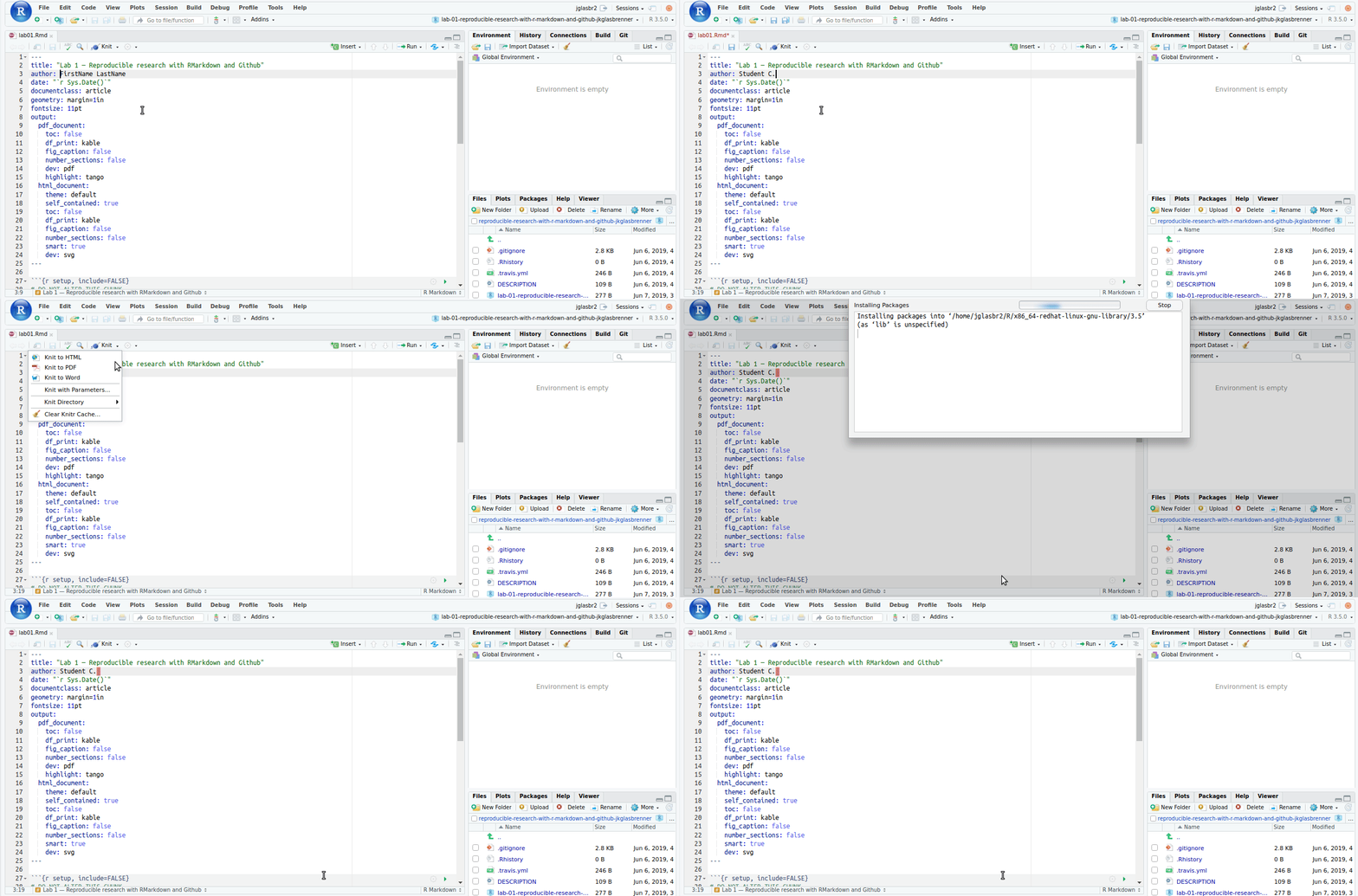
   After knitting is complete, a pop-up window should open. Based on the output that you see, explain what the ## symbols are doing to the text. Write your explanation below This is Exercise 1.

   Pop-up problems

   If you do not see a pop-up after clicking knit, then your web browser is most likely blocking pop-ups. Fix this by telling your browser to allow pop-ups from RStudio Server, here are instructions for  Google Chrome and for  Firefox.

Let’s write some more Markdown and see what it does.

2. Type the markdown text in the box below into your lab report file exactly you see it under ## Exercise 2. Then, knit the file to PDF again and look at the output. Write a short explanation of what each markup symbol does.

   *What happens when you surround text with one-star pairs?*
   
   **What happens when you surround text with two-star pairs?**
   
   ***What happens when you surround text with three-star pairs?***
   
   1.  Start typing this list. Note there are two spaces between the period and the word "Start".
   2.  Type the second line of the list
   1.  What happens if I type step 3 as another step 1?
   
   *   What does this star at the beginning do?
   *   Visually, it's similar to the numbered list.
   
   1.  What happens if we nest a list?
       1.  Type four spaces, then type the number
       2.  Did this do what you expected?
   2.  What if we continue the numbers this way?
       *   What happens if we indent using stars?
       *   Let's add another one for good measure.
           *   Can we get another level of nesting?
   
   [What does this do?](https://google.com)
   
   ![How is this different from the above?](test-image.jpeg)

Interlude: How to save your work back to GitHub

Now that you’ve typed some material into your R Markdown document, let’s take a snapshot of our work using what is called a “commit”. The animation below demonstrates how to do this,

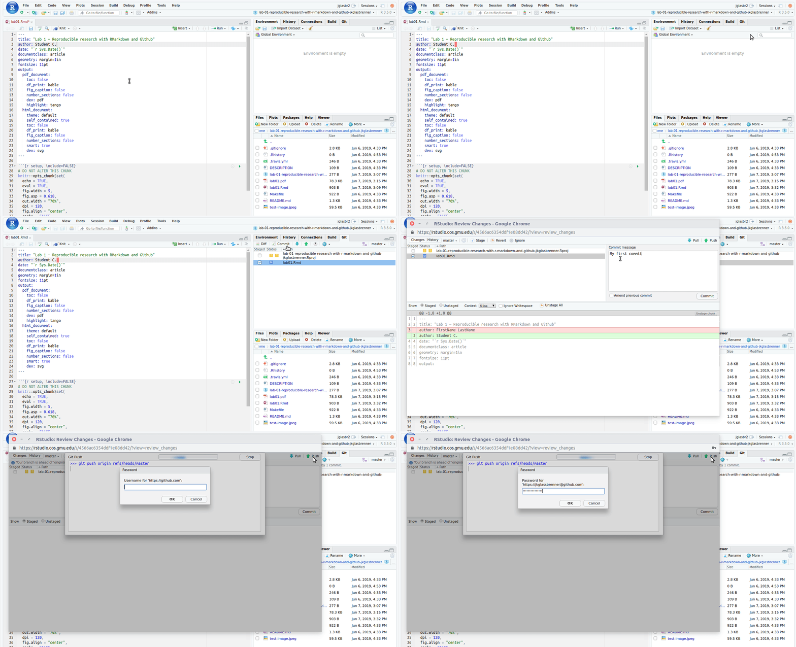
The animation shows the following steps,

• If you haven’t already, save your work by clicking the save icon just above the editing window.

• Go to the Workspace Tabs panel and click the Git tab. You will see a list of files that have been added or changed in the project. Since we changed lab01.Rmd, it is shown in the list.

• To stage the changes made to lab01.Rmd, in the Git tab click the check box to the left of the file.

• Click the button labeled Commit, which will open up a pop-up window. In the pop-up, you should still see a check in the check box to the left of lab01.Rmd.

• Click anywhere in the text box labeled Commit message and then write a brief, informative message there (in the example, the somewhat unhelpful “My first commit!” is used as a message).

• Click the commit button.

After clicking the commit button, you have taken a snapshot of your work. You should notice that lab01.Rmd is no longer listed in the pop-up window or in the Git tab. This means that your commit worked and the snapshot of lab01.Rmd is now up-to-date.

The animation continues from this point and shows you how to perform a “push”. Pushing your changes is how you send your updated files back to GitHub. It is only after completing a push that the course instructor can see your updated files. As shown in the animation, to perform a push after you make a commit, you do the following,

• Click the button labeled Push in the Git pop-up window.

• Fill in your GitHub username and password in the subsequent pop-ups.

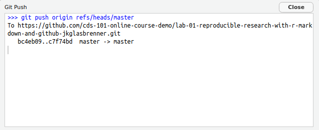
If the push is successful, you will see a message that resembles this one,

More Markdown

Now that we’ve saved and synchronized our work on GitHub, let’s return to R Markdown. During the rest of the lab, you are encouraged to commit early and often. This will help you get more comfortable with this workflow, which you will use for the rest of the semester.

3. You can create tables using Markdown, type in the following and then knit your document to see it looks like. Do both tables look the same after being rendered? What are the lines that start with the word Table: doing?

   | Column 1 | Column 2 | Column 3 | Column 4 |
   | --- | ---: | :---: | :--- |
   | Notice | what | the | colons |
   | are | doing? | | |
   
   Table: The table with poor spacing
   
   | Column 1 | Column 2 | Column 3 | Column 4 |
   | -------- | -------: | :------: | :------- |
   | Notice   | what     | the      | colons   |
   | are      | doing?   |          |          |
   
   Table: The table with good spacing

4. Copy-and-paste one of the above tables and add a fifth column to it. Fill in whatever text you like to create the fifth column.

While formatting text is important, the most powerful feature of R Markdown is that it allows us to write and run code within the document itself. Let’s consider a couple of different commands to demonstrate how this works.

5. Type the following code block into your file, then click the green “play” icon that appears to the right of your code block. Explain what you’re getting as output.

   ```{r}
   qplot(x = displ, y = hwy, data = mpg)
   ```

6. What output do you get if you type the following in a code block? Do you see a connection between certain parts of this output and the one from the previous question? If so, what are they? If not, why isn’t there a connection?

   ```{r}
   print(mpg)
   ```

How to submit

Now that we’re done with Lab 1, we need to prepare our report for submission. Click the save icon and knit your document to PDF. If there are no errors, then a pop-up containing your knitted PDF should appear. Inspect the PDF to make sure that you’ve answered all the questions and check that the formatting for your text, figures, and tables looks good.

To submit your lab, follow the two steps below. Your lab will be graded for credit after you’ve completed both steps!

1. Save, stage, commit, and push your completed R Markdown file so that everything is synchronized to GitHub. If you do this right, then you will be able to view your completed file on the GitHub website. Please note that you won’t be able to commit and push the knitted PDF file.

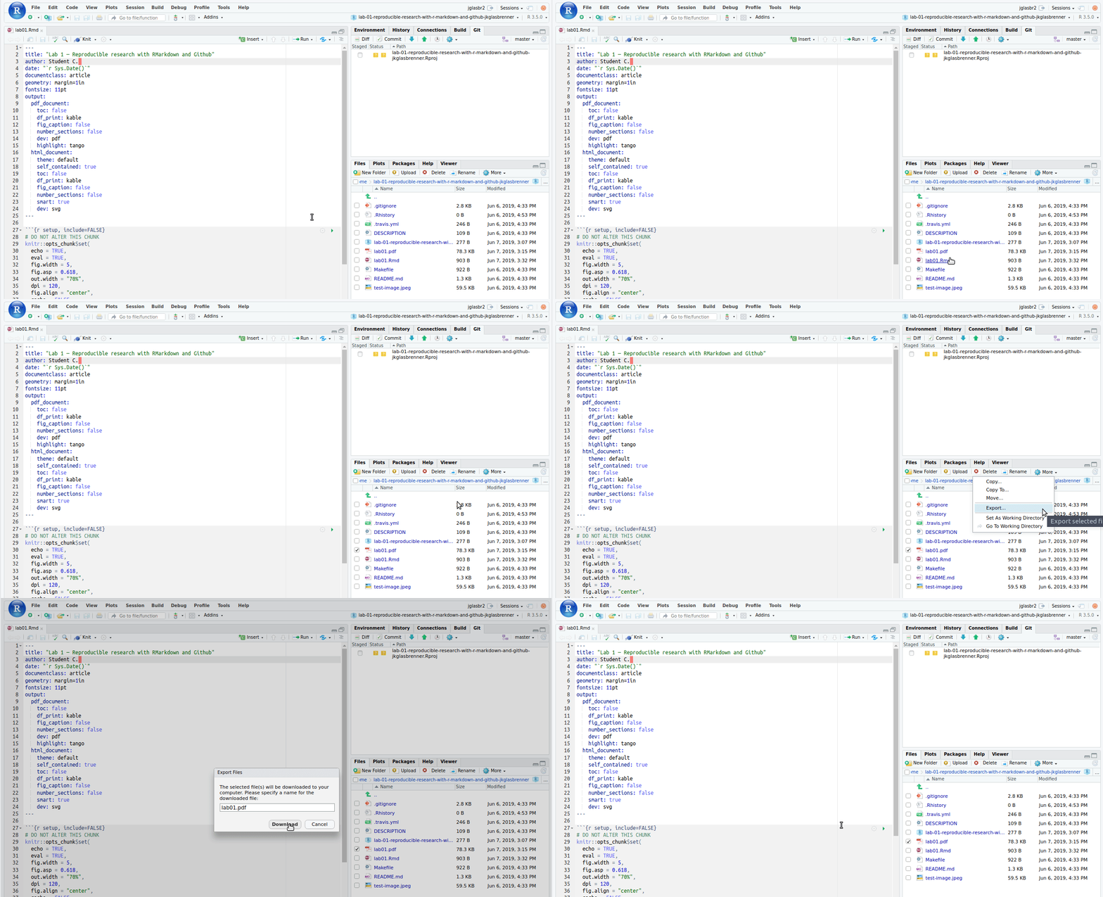
2. Upload your knitted PDF file to Blackboard. To do this, you will first need to download it to your computer. Check the box to the left of lab01.pdf, click the More button, choose Export in the drop-down menu, and click the Download button in the pop-up that appears. This will download the file to your computer, most likely to your Download folder. Locate this file and then submit it to Lab 1 posting on Blackboard.

   

Cheatsheets

Linked below are some official cheatsheets published by RStudio,

• RStudio cheatsheet

• R Markdown cheatsheet

• R Markdown reference

These are a handy reference to have nearby while working on the labs. You may even want to print them out and keep them by your computer as you complete the labs.

Credits

This lab is licensed under a Creative Commons Attribution-NonCommercial-ShareAlike 4.0 International License. Portions of the instructions were adapted by James Glasbrenner from Lab 0 - Introduction to R and RStudio by Mine Çetinkaya-Rundel and the Github Classroom Guide for Students by Jacob Fiksel. The rest of the Exercises and instructions were written by James Glasbrenner for CDS-102.